In the past year I have seen a few press releases by WhiteWater Security (WWS) regarding their WaterWall product:
WaterWallג„¢ is a revolutionary end-to-end water security management system, designed to give decision-makers and water security operators an unprecedented level of decision-making confidence in the event of a water crisis. From prevention and detection to intelligent response and recovery through automatic procedure scenarios, WaterWallג„¢ dramatically improves the speed, reliability and quality of responses vital to successful water security management.
An important part of the WaterWall is something called the BlueBox which is an Event Detection System (EDS). In WWS’s web site there is no information of how this EDS works. Fortunately, I attended a one day conference about SCADA systems held by Lead Control. It turns out that Lead is the developer of the BlueBox module. From bit and pieces of information I’m able to give you the basic algorithm running it all. Please note that this is my understanding of the algorithm and may not truly reflect it in detail.
For the explanation I will be using data sets from the CANARY distribution which is the EPA’s event detection software. The data set includes a time series of six parameters: Cl2, PH, Temperature, Turbidity, TOC and Conductivity.
Step 1 – Normalization
Since every measured parameter has its own units and range all of the readings have to normalized. There are more than one way to normalize data so I have selected to normalize each data set using its mean and standard deviation to obtain a mean of zero and a standard deviation of one. This is done for the selected moving time window. As we steps through each new time step, the oldest data point is removed from the window, the most recent data point is added to the window and the data in the new window is normalized again to create a new mean and standard deviation.
Step 2 – Calculate points distance
At each point in time we have a set of the six parameters. Each of these sets represents a point in a six dimensional space (like x, y and z in three dimensions). The Euclidean distance between each point to all of the others may be calculated.
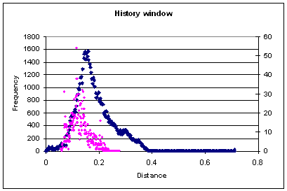
Step 3 – Plot the frequency curve of the distances
Once we have the distances calculated we can easily plot its frequency curve as shown in the following figure:

Step 4 – wait for the next reading
Now we are ready for the next data set to come from the SCADA system. Once a new set of the six parameters arrives we move the history window one time step ahead and calculate the distance of the new point to the points in the history window. And again we plot the distances frequencies on top of the previous curve:

Since the point is “normal”, its frequency distribution is “normal”, meaning its similar to the history distribution. But when an event is detected the new distribution may look like so:

It is clear that the new point’s distance frequency is “far” from the normal distribution. Hence, an event.
Conclusion
The algorithm described here is very simple and that is its beauty. I have written its implementation in about an hour but in order to make it an online module a lot of work is needed. Once developed it may be able to do a number of things:
- identify abnormal behavior.
- identify normal but unusual behavior.
- identify a parameter that is causing the abnormal behavior.
- the system may function with one or more parameters missing.
unusual


